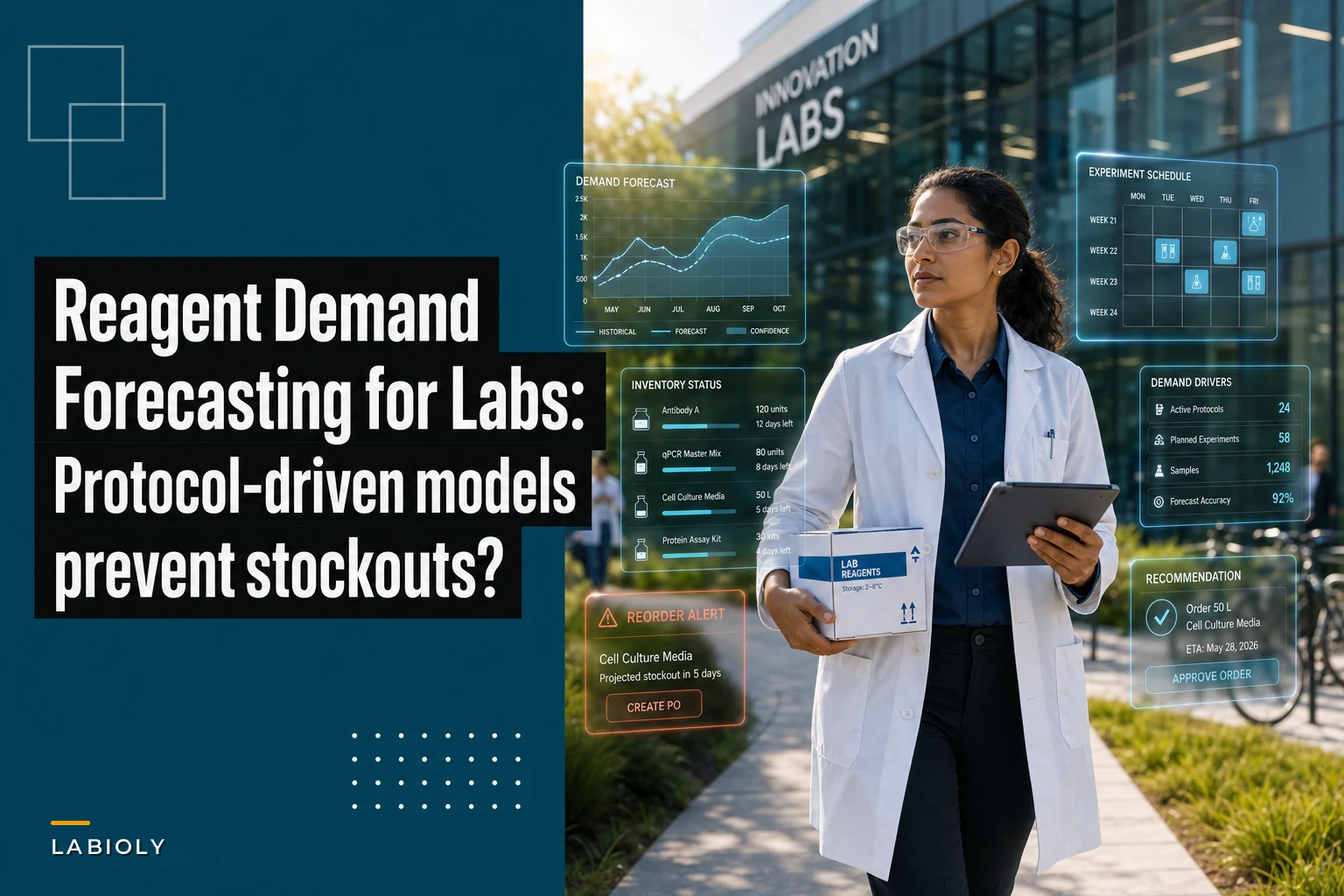
Reagent Demand Forecasting for Research Labs: Protocol-Driven Models to Prevent Stockouts

Build forecasting models that actually match how your lab consumes reagents—not generic inventory formulas from manufacturing

Your lab manager just ordered $18,000 worth of antibodies because the freezer looked empty. Two weeks later, you find three unopened vials hiding behind the PCR reagents—expiring next month. Meanwhile, the RNA extraction kit you actually need for tomorrow's experiment? Backordered six weeks out.

This happens in research labs constantly—not because people are careless, but because traditional inventory forecasting completely falls apart when applied to reagent demand. Manufacturing-style reorder points assume steady consumption. Labs don't work that way.

Why Standard Forecasting Breaks in Research Settings

Research consumption follows experiment schedules, not calendar patterns. A western blot antibody might sit untouched for eight weeks, then suddenly you need 12 vials when three projects hit the validation phase at the same time. Traditional MIN/MAX calculations see eight weeks of zero usage and suggest cutting stock levels—right before your demand spike hits.

The real problem runs deeper than irregular timing. Protocol requirements create rigid consumption blocks. If your ChIP-seq protocol needs exactly 4μg of antibody per sample, you can't stretch it to 3.5μg when supplies get low. You either have enough reagent to complete the full experiment set, or you delay the entire project.

Then there's the grant cycle effect. When an R01 gets approved, you're suddenly scaling from pilot studies to full experimental runs. Your monthly reagent burn rate might jump 400% almost overnight. Standard forecasting models treat this as an outlier to smooth over. For your lab, it's the new normal for the next four years.

Building a Protocol-Driven Forecasting Framework

Instead of tracking historical averages, you build consumption models from your experimental protocols.

Start with your protocol library. For each standard procedure, document the exact reagent requirements—not estimates, actual measured consumption including waste factors. A typical qPCR run might list 20μL per reaction, but after accounting for pipetting loss and dead volume, you're really burning through 24μL.

Map these protocols to your experiment calendar. This isn't about guessing what experiments might happen—it's about tracking what's already scheduled. Most labs plan experiments four to eight weeks out based on sample availability, equipment bookings, and milestone deadlines. That forward visibility becomes your demand forecast.

Here's what this looks like in practice:

Week	Scheduled Experiments	Taq Polymerase Need	DMEM Required	Antibody X
1	3 qPCR plates	450 units	-	-
2	Cell expansion	-	2000 mL	-
3	5 qPCR plates	750 units	500 mL	-
4	Western validation	-	500 mL	25 μg
5	2 qPCR plates	300 units	1000 mL	-

Once you have scheduled demand mapped out, add your baseline consumption—the steady-state usage from maintenance activities. Cell culture media for keeping lines alive, enzymes for routine quality checks, buffers for equipment cleaning. These create your consumption floor.

Visual workflow: mapping protocols to scheduled experiments to predicted reagent demand and reorder triggers.

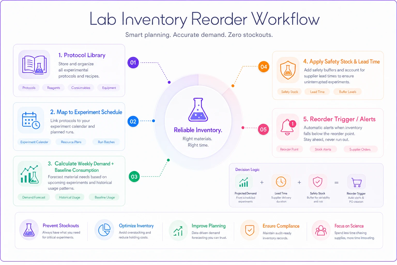
The graphic shows how protocol details and the experiment calendar drive demand estimates and triggers.

Handling Intermittent and Spike Demands

Research labs face two distinct demand patterns that break standard models: true intermittent demand (long stretches of zero usage) and sudden spikes from grant-driven scaling.

For intermittent demand, Croston's method works better than averaging. Instead of dragging all those zero-usage periods into your average, you separately forecast the interval between demands and the quantity when demand actually occurs.

Interval forecast = Average time between non-zero demands Quantity forecast = Average quantity when demand occurs Period forecast = Quantity forecast / Interval forecast

Take that western blot antibody. Over 20 weeks, you used it five times:

Week 3
15 μg
Week 7
20 μg
Week 11
18 μg
Week 14
22 μg
Week 19
17 μg

Average interval: 4 weeks between uses

Average quantity: 18.4 μg per use

Forecast: 4.6 μg per week (18.4 / 4)

Compare that to simple averaging: 92 μg total / 20 weeks = 4.6 μg per week. Same result here, but watch what happens with sparser usage patterns. If you only used the reagent three times in 20 weeks, simple averaging drops your forecast to 2.3 μg per week while Croston's method holds at a more realistic 5.5 μg per week.

For spike demands, you need trigger-based adjustments. When specific events occur—grant approval, new project kickoff, clinical trial phase change—your model shifts to a different consumption level. Build multiple forecast scenarios:

Baseline
Current steady-state
Scale-up
3x consumption for the first 8 weeks of a new project
Full production
5x sustained after validation phase
Wind-down
0.5x during publication and analysis periods

Wind-down: 0.5x during publication and analysis periods

Calculating Safety Stock for Research Operations

Safety stock in labs isn't really about demand variability—it's about the consequences of running out and how long it takes to restock. Missing a reagent can mean:

Losing time-sensitive samples
Breaking longitudinal study continuity
Wasting other expensive reagents from incomplete experiments
Missing grant milestone deadlines

Standard deviation-based safety stock assumes occasional stockouts are acceptable. Research can't absorb that. Instead, calculate based on maximum reasonable demand during lead time, then add a protocol completion buffer.

A practical formula:

Safety Stock = (Max weekly usage × Lead time weeks) + Protocol buffer

Where protocol buffer = Largest single experiment requirement

For Taq polymerase:

Max weekly usage
750 units (from Week 3)
Vendor lead time
2 weeks
Largest protocol
300 units (2 plates)

Safety stock = (750 × 2) + 300 = 1,800 units

This covers maximum demand during the reorder window and leaves enough to complete one full experiment even if delivery slips.

Lead Time Realities and Multi-Vendor Strategies

Published lead times for research reagents are essentially fiction. That "3-5 business days" becomes three weeks when the antibody is custom-conjugated, the vendor's out of stock, or your institution's purchasing department sits on the PO for a week.

Track actual lead times by vendor and product category:

Vendor	Product Type	Quoted Lead	Actual P50	Actual P90
ThermoFisher	Standard enzymes	3-5 days	7 days	14 days
Abcam	Primary antibodies	5-7 days	12 days	28 days
Sigma	Custom peptides	3-4 weeks	5 weeks	8 weeks
Local distributor	Common chemicals	Next day	2 days	5 days

P50 means half your orders arrive within that timeframe. P90 means 90% do. Use P90 for critical reagents, P50 for items where substitutes are available.

For anything critical, split orders across vendors even if it costs more.

When your entire project depends on one antibody, paying a 20% premium for a backup source is cheap insurance against a six-week delay from a single vendor stockout.

Spreadsheet Implementation with Worked Examples

Sheet 1: Protocol Consumption Library

Protocol ID	Protocol Name	Reagent	Quantity per Run	Waste Factor	Total per Run
P001	96-well ELISA	Detection Ab	5 mL	1.15	5.75 mL
P001	96-well ELISA	Substrate	12 mL	1.10	13.2 mL
P002	qPCR standard	Taq Master Mix	1.5 mL	1.20	1.8 mL
P003	T75 passage	DMEM	30 mL	1.05	31.5 mL

Sheet 2: Experiment Schedule

Week Start	Project	Protocol	Runs	Priority
Nov 4	Cancer screen	P001	3	Critical
Nov 4	Maintenance	P003	5	Standard
Nov 11	Gene expression	P002	8	High
Nov 11	Cancer screen	P001	2	Critical

Sheet 3: Demand Calculation

=SUMIFS( ConsumptionLibrary[Total per Run], ConsumptionLibrary[Reagent], "Detection Ab", ExperimentSchedule[Week Start], DATE(2024,11,4) ) * ExperimentSchedule[Runs]

This gives you:

Week Nov 4
Detection Ab needed = 5.75 mL × 3 runs = 17.25 mL
Week Nov 11
Detection Ab needed = 5.75 mL × 2 runs = 11.5 mL

Sheet 4: Reorder Triggers

Reorder Point = (Total demand over lead time) + Safety stock Days until reorder = (Current stock - Reorder point) / Average daily usage

For Detection Ab with 45 mL current stock:

Lead time
14 days (P90 for critical reagent)
Demand next 14 days
28.75 mL
Safety stock
17.25 mL (largest weekly usage)

Reorder today (current 45 mL < reorder point 46 mL)

Implementing Exception Detection and Alerting Rules

The spreadsheet gives you the numbers, but you need exception logic to catch problems before they become project blockers. Build alerts for these patterns:

Insufficient stock for scheduled experiment: When inventory won't cover a specific upcoming protocol, even if overall levels look fine. That 50 mL of antibody means nothing if tomorrow's experiment needs 60 mL.

Lead time violations: When time-to-reorder-point is shorter than vendor lead time. If you'll hit your reorder point in 5 days but the vendor needs 14, you're already behind.

Expiration waste risk: When current inventory will expire before it gets used. This happens constantly with sera and growth factors—you maintain stock levels that look fine on paper, but the reagents degrade before the demand arrives.

Grant-driven demand shifts: When upcoming project changes will invalidate your current forecasts. Flag whenever new grants, collaborations, or scale-up decisions will push consumption beyond what the current model accounts for.

In practice, one of these alerts might look like:

=IF( CurrentStock - NextProtocolRequirement < 0, "BLOCKING: Insufficient for " & NextExperiment_Name, "OK" )

The alerts need to be actionable and tied to responsibility—who places the order, who approves emergency purchases, and who reroutes experiments if needed.

Automation Opportunities and Workflow Integration

The protocol-driven forecasting model outlined above works, but maintaining it manually across 200+ reagents turns into a part-time job on its own. Experiment schedules live in one system, inventory in another, and somehow you need to keep both in sync with purchasing. That coordination gap is where things fall apart.

Operational software with AI automation changes this dynamic. Instead of manually copying protocol requirements into spreadsheets, the system reads your electronic lab notebook entries and maps upcoming experiments to reagent needs automatically. When someone books equipment time for next Thursday's qPCR run, the platform already knows that means 750 units of polymerase need to be on hand by Tuesday.

The more useful capability comes over time. After tracking actual versus projected consumption for several months, AI-assisted platforms can identify where your waste factors are off, which vendors consistently deliver late, and when certain projects tend to exceed planned usage. Forecasts adjust based on those patterns without someone having to manually recalibrate the model every quarter.

The exception monitoring piece matters too. Rather than checking spreadsheets every morning for reorder triggers, the system watches all parameters continuously and only surfaces alerts when action is actually needed—and it can differentiate between "place an order this week to stay ahead" and "this will block Thursday's experiment if you don't act today."

Most of the data you'd need is already sitting in your lab's systems—protocol documents, equipment calendars, inventory databases. An automated platform just removes the manual work of connecting them.

Making This Work in Your Lab

Start with your highest-value reagents—the ones where a stockout actually hurts. Build the protocol consumption model for 10 to 15 items first. Track forecast accuracy for a month before expanding.

Get your lab members to commit to scheduling experiments at least two weeks out. Researchers push back on rigid planning, but framing it as "making sure your reagents are ready when you need them" lands better than calling it administrative process.

Some variation is unavoidable. Your model might accurately predict around 80% of demand. That's still considerably better than the 40% accuracy you get from traditional min/max ordering—and the protocol-based approach at least tells you which 20% is uncertain.

For labs running fewer than 50 experiments a month, the spreadsheet approach works fine with weekly updates. Beyond that scale, you need either dedicated staff maintaining the forecasts or operational software handling the calculations. The cost of one expired antibody kit usually justifies either.

Reagent forecasting in research isn't about minimizing inventory costs the way manufacturing does it. It's about protecting experimental continuity. A couple hundred dollars in additional monthly carrying costs is nothing compared to a three-month publication delay from a stockout.

The protocol-driven model aligns your inventory with how research actually works—in experimental blocks, not smooth consumption curves. Once you stop fighting the inherent lumpiness of lab demand and start planning around it, the emergency orders and expired reagents become occasional exceptions rather than a weekly headache.