

You're running a 48-hour enzyme kinetics study. Everything looks normal until hour 36, when your absorbance readings drop 15%. The plate reader has been drifting since hour 12—you just didn't know because nobody was tracking control samples between runs. Now you've lost three days of work and have to repeat the whole experiment.
This is what calibration drift detection labs deal with constantly. The problem isn't that instruments drift—they all do. The problem is most labs only find out after the damage is done. By the time you notice weird results in your research samples, it's already spread across multiple experiments, multiple users, maybe multiple weeks.
Control-sample scheduling paired with statistical checks catches drift while you can still do something about it. Not the basic "run a standard once a day" approach most labs use, but actual statistical process control adapted for research instruments. The kind that triggers maintenance before drift ruins experiments, not after.
Why Traditional QC Misses Gradual Drift
Most labs run quality control samples at fixed intervals—start of day, maybe between batches. That catches sudden failures but completely misses slow drift. A spectrophotometer losing 0.5% sensitivity per week looks fine in daily checks. Eight weeks later, you're down 4% and wondering why your protein concentrations seem off.
The bigger issue is how labs handle control data. They check if values fall within range but ignore trends. A control reading of 98 on Monday and 92 on Friday both pass a 90–110 acceptance range. Nobody notices the downward pattern until it breaks through the lower limit.
Research labs compound this by running different methods on the same instrument. Your nucleic acid quantification might use 260nm while protein assays run at 280nm. Drift affects wavelengths differently, so a problem showing up in one application might be completely invisible in another. Without wavelength-specific controls, you're missing half the picture.
Then there's the human factor. When a control fails, the usual response is to rerun it. If it passes the second time, most people move on. But that first failure was telling you something—humidity spiked, someone bumped the instrument, there's an intermittent electrical issue. These warning signs get buried in lab notebooks and never analyzed as patterns.
Here's a simple breakdown of how traditional QC compares to statistical monitoring:
| QC Approach | What It Catches | What It Misses |
|---|---|---|
| Fixed interval controls | Sudden failures | Gradual drift |
| Range-based acceptance | Out-of-range values | Directional trends |
| Single wavelength checks | Method-specific issues | Cross-wavelength drift |
| Manual log review | Documented failures | Buried warning patterns |
| Statistical process control | Trends, shifts, patterns | Nothing, if run correctly |
The bigger issue is how labs handle control data. They check if values fall within range but ignore trends. A control reading of 98 on Monday and 92 on Friday both pass a 90–110 acceptance range. Nobody notices the downward pattern until it breaks through the lower limit.
Statistical Rules That Actually Work in Research Settings
Forget the complex SPC charts from manufacturing. Research labs need simpler rules that hold up with smaller sample sizes and varied experimental conditions. Three statistical checks cover most drift patterns you'll actually encounter.
Eliminate lab bottlenecks and errors.
Labioly helps you monitor, manage, and report lab activities efficiently and compliantly.
- Real-time sample tracking
- Inventory and supply alerts
- Staff workflow coordination
No credit card required
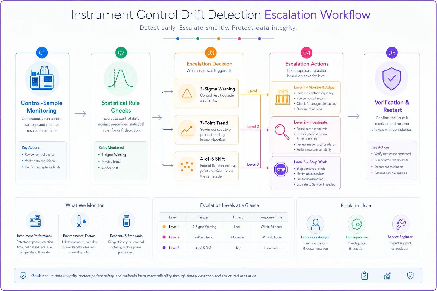
First, the 2-sigma warning rule. Calculate your control mean and standard deviation from the last 20 measurements. When a new control falls between 2 and 3 standard deviations from the mean, that's a warning. Don't stop work yet, but increase control frequency for the next five runs. This catches drift before it actually affects your data.
Second, the trend rule. Seven consecutive control readings moving in the same direction indicates systematic drift—even if all the values technically pass your acceptance criteria. Something is changing: lamp aging, detector sensitivity, optical alignment. The earlier you catch it, the easier the fix.
Third, the shift rule. When four out of five consecutive controls fall on the same side of the mean, something shifted. Maybe someone adjusted a setting without documenting it, maybe room temperature changed, maybe you switched reagent lots. This rule catches step changes that would never trigger a range violation.
The key is combining these rules. A single 2-sigma warning might just be random noise. But a 2-sigma warning followed by three readings above the mean? That's a real signal. The pattern matters more than any individual value.
For shared instruments, track controls by operator. One person's controls might trend upward while everyone else's stay flat. That usually means technique differences—pipetting angle, sample mixing, timing. Catching operator-specific patterns early prevents those "why can't anyone else reproduce my results" situations.
Control Frequency Based on Instrument Stability
Not every instrument needs the same monitoring schedule. A mass spec running around the clock needs different controls than a PCR machine used twice a week. Base your frequency on three things: historical stability data, usage patterns, and how badly drift would affect your experiments.
Start by pulling six months of control data. Calculate the CV for each instrument-method combination. Under 2% CV means you can use longer intervals between controls. Above 5% means tighter monitoring—controls every four samples instead of every twenty.
Usage patterns matter because drift usually correlates with run time, not calendar time. A plate reader running 200 plates per week degrades faster than one running 20. Track drift rate per operational hour, not per day. That gives you maintenance intervals based on actual wear.
Some applications also tolerate more drift than others. Screening assays looking for 2-fold changes can handle 5% drift without much consequence. Quantitative assays measuring 10% differences need drift below 1%. Match your control frequency to your experimental requirements, not just the instrument's specs.
A practical framework that works across most research labs:
-
High-stability instruments (CV <2%) - Daily
Single control at startup - Per batch: Control every 20–30 samples - Weekly: Full calibration verification
-
Medium-stability instruments (CV 2–5%) - Shift-based
Control at start and mid-shift - Per batch: Control every 10–15 samples - Twice weekly: Calibration check
-
Low-stability instruments (CV >5%) - Continuous
Control every 5–8 samples - Hourly: Dedicated control run - Daily: Calibration adjustment if needed
Temperature-sensitive instruments often need seasonal adjustments too. A fluorometer that's rock-solid in winter might drift constantly during summer humidity. Track seasonal patterns and adjust accordingly.
Escalation Triggers and Response Protocols
When controls fail statistical checks, you need clear escalation paths. Not every deviation warrants the same response. A structured protocol prevents both under-reaction (ignoring real problems) and over-reaction (unnecessary shutdowns that kill productivity).
Level 1: Warning (2-sigma rule triggered)
Response time: Immediate
-
Flag current batch for review
-
Increase control frequency to every 5 samples
-
Document in instrument log
-
Continue operations with heightened monitoring
-
If next 5 controls pass, return to normal frequency
Level 2: Investigation Required (trend or shift detected)
Response time: Within 2 hours
-
Complete current critical samples only
-
Run verification controls at multiple concentrations
-
Check environmental conditions (temperature, humidity, vibration)
-
Review recent maintenance or any changes made
-
Document findings and corrective action
-
Must pass verification before resuming normal operations
Level 3: Stop Work (3-sigma violation or multiple rules triggered)
Response time: Immediate stop
-
Halt all sample processing
-
Tag all affected runs for possible re-analysis
-
Perform root cause investigation
-
May require recalibration or service call
-
Must pass full verification protocol before restart
The investigation process matters as much as the trigger levels. When drift shows up, check these factors in order:
Environmental changes first—someone may have moved the instrument near an air vent or window. Easy to fix if caught early, maddening if ignored for weeks.
Then consumables. New lot of cuvettes with slightly different optical properties? Different supplier for control materials? Reagent approaching expiration? These create step changes that look exactly like instrument problems.
Finally, usage patterns. Did someone run an unusual method that changed instrument settings? Was there a power interruption? Did maintenance clean something they shouldn't have? The instrument log should capture these events, but often doesn't.
The escalation workflow looks like this:
Building these escalation rules into your operational software is where things get genuinely useful. When control data streams into your QC system, statistical checks can run automatically in the background. AI automation handles pattern detection across multiple instruments at once, flagging things a person would likely miss—like three instruments drifting simultaneously, which points to an environmental cause rather than three independent failures.
Verification Runs That Validate Fixes
After addressing drift, you need proof the fix actually worked. Running one control and calling it done isn't enough. Verification runs should stress-test the instrument across its full operational range.
Start with a bracketing approach. Run controls at roughly 20%, 50%, and 80% of your typical measurement range. If you normally measure proteins at 0.5–2.0 mg/mL, verify at 0.4, 1.0, and 1.6 mg/mL. This confirms linearity wasn't affected by whatever caused the drift.
-
Basic Verification (after Level 1 warnings) - Run three replicate controls at working concentration - Confirm CV <3% - Document in instrument log - Resume normal operations
-
Standard Verification (after drift correction) - Bracketing test: Low, medium, high concentration controls - Each concentration in triplicate - Confirm linearity R² >0.99 - All CVs <3% - Document corrective action and results
-
Comprehensive Verification (after major maintenance) - Full calibration with fresh standards - Bracketing test across full range - Method-specific controls for each application - Time stability test (4-hour run) - Inter-operator comparison if multi-user instrument - Generate new control limits from 20 measurements
Keep verification data separate from routine control data. Post-maintenance adjustments can skew your control statistics if mixed in. After major work, establish new baseline statistics rather than trying to maintain historical continuity.
Connecting Drift Patterns to Root Causes
Different drift patterns point to different problems. Learning to read them turns reactive maintenance into something closer to predictive.
Linear drift usually means component aging. Lamp intensity decreases predictably, detector sensitivity degrades gradually. These are easy to model—track the drift rate and schedule preventive maintenance before it starts affecting data quality.
| Drift Pattern | Likely Cause | Priority |
|---|---|---|
| Linear decline | Component aging (lamp, detector) | Schedule preventive maintenance |
| Step change | Discrete event (cleaning, reagent lot, settings) | Investigate immediately |
| Cyclic variation | Environmental (HVAC, temperature, vibration) | Correlate with facility data |
| Increasing variation | Mechanical wear | Inspect before failure |
| Sudden improvement | Undocumented change | Investigate and document |
Step changes indicate discrete events: someone cleaned the optics, you switched reagent lots, facilities adjusted the building temperature. These usually have simple fixes, but the key is catching them immediately rather than weeks later.
Cyclic patterns suggest environmental factors. Daily temperature swings, HVAC cycling, building vibration from nearby construction. Plot your control data with timestamps and look for patterns that match building operations. One lab traced their morning drift to a parking garage gate opening and causing vibrations through the building structure—not something you'd ever guess without that data.
Increasing variation without mean shift is a warning sign for mechanical wear. Bearings loosening, optical mounts degrading, electrical connections oxidizing. The instrument still hits the target on average, but precision decreases. This pattern tends to predict catastrophic failure—worth fixing before it becomes a crisis.
Sudden improvement also needs investigation. If controls abruptly get tighter or shift to better values, something changed. Maybe someone finally cleaned something, maybe they adjusted a setting without documenting it. Improvements aren't automatically good news—they mean something unknown happened to your instrument.
Real Implementation: Academic Core Facility
A university proteomics core was dealing with constant complaints about irreproducible results between users. They ran daily controls but kept missing user-specific problems. Different postdocs were getting different results from identical samples.
They implemented statistical control monitoring with user-tagged controls. Each user ran a control at session start and every 10 samples. The data fed automatically into their tracking system, which calculated user-specific control limits.
Within two weeks, patterns emerged. One user's controls ran consistently 8% high; another's showed double the normal variation. Investigation revealed technique differences—one person vortexed samples differently, another let samples warm up longer before reading.
The more interesting discovery was instrument-specific drift signatures. Their oldest mass spec showed logarithmic drift after cleaning, taking roughly three days to stabilize. Their newest showed step changes whenever lab temperature dropped below 68°F. These patterns were invisible in averaged daily controls but obvious in continuous statistical monitoring.
-
User variation >5% triggered retraining
-
Instrument trend over 7 consecutive points scheduled maintenance
-
Environmental correlation prompted HVAC setting adjustments
-
Post-cleaning instability triggered an extended stabilization period before normal operations resumed
Results after six months:
-
User complaints dropped roughly 75%
-
Repeat runs decreased from around 20% to under 5%
-
Maintenance costs stayed flat—better scheduling offset increased frequency
-
Audit findings on data quality went from 3–4 per audit to zero
The key wasn't running more controls—they actually ran fewer than before. The difference was running smart controls with statistical analysis and clear response protocols.
Software Makes Statistical Monitoring Scalable
Manual control charting works for one or two instruments. Beyond that, you need operational software that handles the statistics automatically. Not just calculating means and standard deviations, but detecting patterns, triggering escalations, and maintaining audit trails.
The practical challenge is connecting instrument data streams, especially from older equipment. Modern instruments might export to LIMS, but that 15-year-old spectrophotometer probably doesn't. You need middleware that captures data regardless of source—CSV exports, manual entry, direct connections, even OCR from printed reports.
Once data flows in, AI automation handles the statistical work continuously. It calculates control limits, checks rules, identifies patterns across instruments, and correlates with environmental data. When drift is detected, it triggers the right workflows—scheduling maintenance, notifying users, requiring verification runs before operations resume.
The longer-term value comes from pattern learning. After monitoring instruments across different lab environments over time, the system starts recognizing failure signatures before they become problems. That specific combination of increasing variation plus a slight mean shift? It might predict pump failure a few weeks out. These predictions improve as more data accumulates.
That said, software can't fix bad processes. If your controls aren't representative of actual samples, perfect statistics accomplish nothing. If people ignore warnings, automated escalation is just noise. The technology amplifies good practices—it doesn't substitute for them.
Calibration drift will always be part of running a research lab. Instruments age, components wear, environments change. The question isn't whether drift will happen but whether you'll catch it before it ruins experiments.
Statistical control monitoring turns drift from a crisis into a managed variable. Instead of discovering problems through failed experiments, you detect them through control patterns. Instead of reactive troubleshooting after the fact, you get predictive maintenance before researchers notice anything.
The framework isn't complicated: run controls based on instrument stability, apply statistical rules to detect patterns early, escalate appropriately when rules trigger, and actually verify that fixes worked. Each piece supports the others. Frequent controls without statistics just generates noise. Statistics without verification documents problems without solving them.
Most labs already have most of the data they need. They run controls, maintain logs, track failures. What's missing is systematic analysis that turns that data into operational intelligence. Whether through manual charting or automated software, the goal is the same: catch drift while it's still fixable, not after it's already cost you a week of research.
The labs that get this right treat control data as operational intelligence, not a compliance checkbox. They know their instruments' normal behavior, recognize deviation patterns, and fix problems before researchers even notice. That's the difference between constantly fighting fires and actually preventing them.
Ready to upgrade your lab operations?
Join 500+ labs using Labioly to save time, reduce errors, and enhance productivity and compliance.